A geometrical interpretation of variational methods in machine learning

Variational methods are often introduced through information theory: learning means finding an approximate distribution that remains close to a target Bayesian posterior. This has a geometrical interpretation. The mathematical object being optimized is not a point in a Euclidean parameter space, it's a probability distribution living on a curved statistical manifold.

This distinction matters because Euclidean distance between parameters does not necessarily measure how much the model changes. Two parameter vectors can be far apart in coordinates while inducing nearly identical distributions. Conversely, a small parameter perturbation can strongly change the predictive behaviour of the model. Variational learning is better understood as motion in a space of distributions.

The Fisher Information Matrix as a local geometry

Consider a parametric family \(q_{\boldsymbol{\theta}}(\boldsymbol{\omega})\), where \(\boldsymbol{\theta}\) parameterizes a distribution over model parameters \(\boldsymbol{\omega}\). The space of such distributions can be viewed as a Riemannian manifold equipped with the Fisher-Rao metric. Infinitesimally, the Kullback-Leibler divergence between two nearby distributions behaves like a squared distance [1,2]:

Here, \(\mathbf{F}(\boldsymbol{\theta})\) is the Fisher Information Matrix:

The Fisher matrix defines the local notion of distance on the statistical manifold. It measures how sensitive the induced distribution is to a change in coordinates. Large Fisher values indicate directions where small parameter changes strongly modify the distribution. Small Fisher values indicate directions where the distribution is nearly insensitive to perturbations [1,2].

Parameter displacement is not distributional change

The Fisher-Rao metric is invariant to reparameterization: it describes the geometry of the distribution itself, not the arbitrary coordinates used to represent it [2,3].

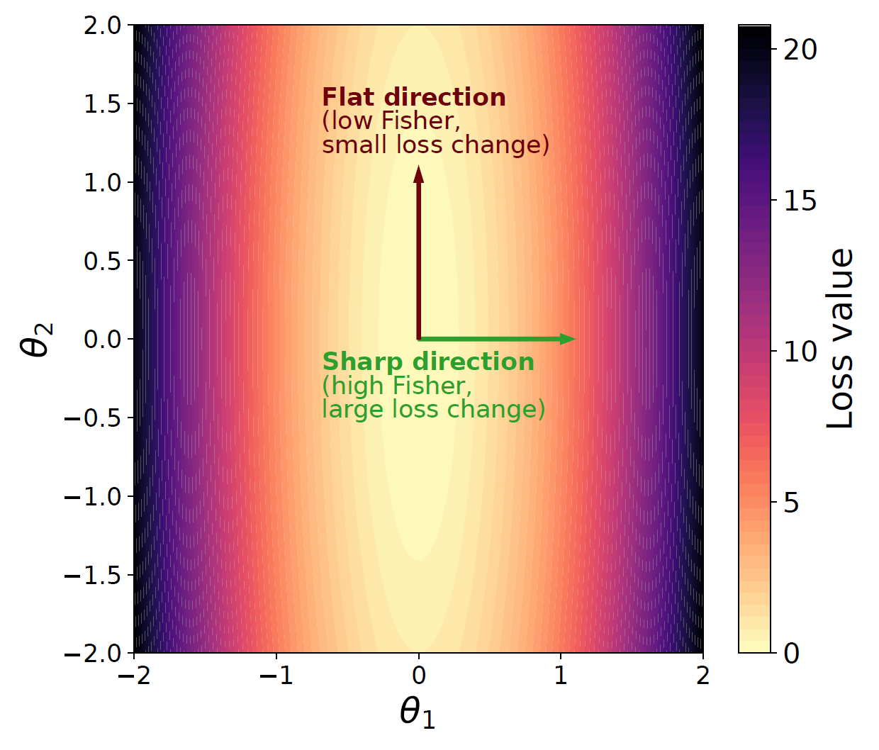
The figure illustrates the anisotropic nature of the loss landscape. Some directions are stiff: moving along them quickly changes the objective and the predictive distribution: this is where the Fisher matrix is large. Other directions are flat: parameters can move without strongly affecting the model. The Fisher geometry expands sensitive directions and contracts insensitive ones, providing a local measure of parameter importance [3].

Natural gradients: optimization in distribution space

This geometry changes the meaning of optimization. In ordinary gradient descent, the steepest direction is defined with respect to Euclidean distance, with a fixed learning rate. In variational inference, the steepest direction is measured with respect to distributional change. In this setting, the natural gradient represents the optimal step. It is obtained by minimizing the first-order variation of an objective \(\mathcal{L}\) under a local KL constraint [1,2]:

Solving this constrained problem gives the natural-gradient direction:

The multiplication by \(\mathbf{F}^{-1}\) corrects the gradient by the local curvature of the statistical manifold. Directions that strongly affect the distribution are scaled down, while flatter directions can be explored more freely [1,2].

Bayesian learning as geometrical optimization

The Bayesian Learning Rule frames several optimization and inference algorithms as updates over approximate posterior distributions. In this formulation, learning is expressed as the minimization of a generalized Bayesian objective, and the resulting updates can be written in natural-parameter space using natural gradients. The Fisher Information Matrix then appears as the metric that makes the update respect the geometry of the posterior family [4].

This is directly connected to continual learning. In methods such as Elastic Weight Consolidation, the Fisher Information Matrix is used to estimate how important each parameter was for a previously learned task. A parameter with a large Fisher value is treated as sensitive: changing it is expected to strongly affect the model's previous predictions. EWC adds a quadratic penalty that discourages such changes. This protects past knowledge, but it also hinders learning by reducing plasticity in directions considered important [5].

Fisher-based continual learning can be interpreted as a geometrical constraint on learning, where the objective adapts to incoming data while limiting changes along directions that would strongly modify the model's learned distribution. Importance is therefore a measure of how costly a parameter perturbation is for the distribution represented by the model [1,2,4,5,7].

MESU: uncertainty shapes the geometry of continual learning

This connection between Bayesian learning and geometry is a main aspect of Metaplasticity from Synaptic Uncertainty (MESU) [6]. In MESU, each parameter is represented by a Gaussian distribution whose variance encodes synaptic uncertainty. The update rule scales learning by this variance: uncertain weights move more easily, while confident weights are stabilized. The posterior geometry directly controls the update.

Continual learning becomes a geometrical compromise between three forces. The likelihood term pulls the posterior distribution toward the new data. The previous posterior preserves directions that have already been constrained by past evidence. The forgetting term relaxes obsolete constraints, preventing the model from becoming overconfident and rigid. Learning, stability, and forgetting therefore act on the same distributional space: learning reshapes the posterior, stability preserves selected directions, and forgetting reopens degrees of freedom for future tasks.

The supplementary analysis makes this link explicit through the Hessian. In the long-time limit, MESU's synaptic variances become inversely related to the diagonal Hessian. High-curvature directions correspond to low variance: the model is confident there, and updates are naturally damped. Low-curvature directions keep larger variance: the model remains uncertain there, and plasticity is preserved. Uncertainty therefore becomes a curvature-aware measure of parameter importance.

This places MESU close to Hessian-based regularization methods such as EWC and SI, but the mechanism is different. EWC and SI estimate parameter importance and impose an external constraint to protect important directions. MESU instead lets importance emerge from the posterior. The same quantity that expresses uncertainty also modulates plasticity and approximates curvature. Stability is not added as a separate penalty; it is induced by the evolving geometry of the Bayesian posterior.

The memory window \(N\) controls how much of the past keeps shaping this geometry. A large \(N\) retains more past information and strengthens consolidation, but it can also collapse variances and reduce plasticity. A smaller or finite \(N\) allows older constraints to fade, keeping part of the parameter space uncertain and available for new information. This gives MESU a direct geometrical interpretation of the stability-plasticity trade-off: continual learning depends on how much the posterior manifold is allowed to contract around past solutions, and how much it remains open for future ones.

This gives intuition about why Bayesian continual learning without forgetting can fail through catastrophic remembering. If all past evidence is accumulated indefinitely, the posterior can become too concentrated. The geometry then contracts in too many directions: gradients are damped, uncertainty vanishes, and the model loses the ability to adapt.

Conclusion

The geometrical interpretation of variational learning provides a unified way to understand natural gradients, Bayesian posterior updates, and importance-based continual learning. The central object is not the Euclidean displacement of parameters, but the distributional change induced by an update. Fisher information, Hessian curvature, and posterior uncertainty are different ways of describing how sensitive the model is along each direction.

References

1. Shun-ichi Amari, Neural Learning in Structured Parameter Spaces — Natural Riemannian Gradient, 1996, Advances in Neural Information Processing Systems.
2. Shun-ichi Amari, Natural Gradient Works Efficiently in Learning, 1998, Neural Computation.
3. Razvan Pascanu and Yoshua Bengio, Revisiting Natural Gradient for Deep Networks, 2014, International Conference on Learning Representations.
4. Mohammad Emtiyaz Khan and Håvard Rue, The Bayesian Learning Rule, 2023, Journal of Machine Learning Research.
5. James Kirkpatrick et al., Overcoming Catastrophic Forgetting in Neural Networks, 2017, Proceedings of the National Academy of Sciences.
6. Djohan Bonnet, Kellian Cottart, Tifenn Hirtzlin, Tarcisius Januel, Thomas Dalgaty, Elisa Vianello, and Damien Querlioz, Bayesian Continual Learning and Forgetting in Neural Networks, 2025, Nature Communications.
7. Ishan Garg et al., Fisher-Orthogonal Projected Natural Gradient Descent for Continual Learning, 2026, arXiv preprint.